They grow up so fast
It’s been at least a year since I last dabbled in TensorFlow, and the ecosystem seems to have grown a lot. The general trend is towards higher-level abstractions for building models, defining data pipelines or serving predictions. Then there is also the relentless community-driven development, spawning many useful extensions to the official library. Yet, using TensorFlow still has a bit of going down into the trenches feel to it compared to fitting your regular ML model in sci-kit learn.
In this post, we will try out a few of the new tools to see how fast we can build a transfer learning model in native TensorFlow. In particular, we will look at the relatively new Dataset API for data ingestion and transformation; and secondly, use tensornets for transfer learning. The library has many pretrained models available and a seemingly easy-to-use syntax.
Transfer Learning 101
Transfer learning is the practice of taking pre-trained models and re-purposing them for a new task without having to retrain the entire network from scratch. One area this approach has been proven extremely effective in is object detection. We can take a network trained on tens of millions of images to predict hundreds of different objects, and modify it to fit our use case.
There are two main flavors of transfer learning: feature extraction and fine-tuning. In case of the former, we remove the last fully-connected layer and treat the rest of the network as a fixed feature extractor. In other words, we freeze the previously learned weights and only train the last layer outputting class probabilities.
In case of fine-tuning, not only do we retrain the classifier at the end of the network, but also the previous layers. You can fine-tune the last couple of layers or the entire network. The choice depends on the similarity of your dataset to what the network was originally trained on, and how much data and patience you have.
And now, Tensornets
There is a long list of pre-trained models to choose from for object detection. Thanks to extensive research in the area performance have been skyrocketing. The latest models can detect 1,000 different objects in a regular picture with 95% accuracy.
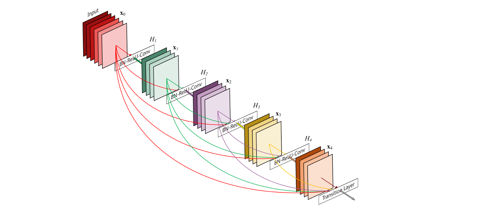
For this particular project I picked dense convolutional networks (DenseNets in short), for no obvious reason other than being the example on tensornets’ GitHub repo. But now that we here: DenseNets are like convolutional networks with the main difference that each layer serves as an input to all subsequent layers. With regular CNN’s each layer is only connected to the following one. According to the paper from 2016:
DenseNets have several compelling advantages: they alleviate the vanishing-gradient problem, strengthen feature propagation, encourage feature reuse, and substantially reduce the number of parameters. 1

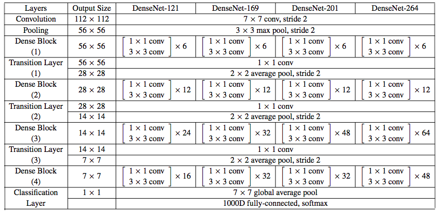
And here is the architecture of the different DenseNets.

Doing transfer learning with DenseNets is as easy as the below according to the package README.
import tensorflow as tf
import tensornets as nets

inputs=tf.placeholder(tf.float32, [None, 224, 224, 3])
outputs=tf.placeholder(tf.float32, [None, 7]) # nr of classes
model=nets.DenseNet169(inputs, is_training=True, classes=7)

loss=tf.losses.softmax_cross_entropy(outputs, model.logits)
train=tf.train.AdamOptimizer(learning_rate=1e-5).minimize(loss)

with tf.Session() as sess:
    sess.run(model.pretrained())
    for (x, y) in your_data:  # the NHWC and one-hot format
        sess.run(train, feed_dict={inputs: x, outputs: y})
If you have seen TensorFlow code, this looks quite straightforward. However, there is a few gotchas when implementing this IRL. Transfer learning has different flavors, and the above is an example of fine-tuning the entire network. That is to say, all updates are going to be backpropagated to all layers. If we wish to freeze some layers, we can pass the list of weights we do want to train to the minimize() method of the optimizer: .minimize(loss,var_list=train_list).
Secondly, keep in mind that the input tensor size is fixed, so we’ll need to reshape our images to fit 224*224*3. The output tensor shape on the other hand can be changed to equal the number of classes in our specific use case.
Thirdly, we need to set the is_training= flag to True during training and to False during testing. Under the hood, this points to the argument of the same name for the batch normalization layers. These layers are responsible for normalizing activations based on the statistics of each batch during training.
However, during test time not only do we need to turn it off, we also need the global statistics (moving_mean and moving_variance) from all batches to use as constants. Somewhat strangely, these values don’t get updated during training by default, and we are left with the statistics of the last batch. This needs to be fixed.
Hence, a more realistic scenario including both training and testing ops would look something like this:
inputs=tf.placeholder(tf.float32, [None, 224, 224, 3])
outputs=tf.placeholder(tf.float32, [None, 7]) # nr of classes
is_train=tf.placeholder_with_default(False, shape=(), name="is_train") # placeholder for is_training

model=nets.DenseNet169(inputs, is_training=is_train, classes=7)
train_list=model.get_weights() # get list of weights
loss=tf.losses.softmax_cross_entropy(outputs, model.logits)

accuracy, accuracy_op=tf.metrics.accuracy(tf.argmax(outputs, 1),tf.argmax(inputs,1)) # local vars

update_ops=tf.get_collection(tf.GraphKeys.UPDATE_OPS) # update batch stats during training
with tf.control_dependencies(update_ops):               # only train last "block"
    train=tf.train.AdamOptimizer(1e-5).minimize(loss, train_list[520:])

init_op=tf.global_variables_initializer()
local_init_op=tf.local_variables_initializer()

with tf.Session() as sess:
    sess.run(init_op)
    sess.run(local_init_op)
    sess.run(model.pretrained())

    for epoch in range(10):
       for (x, y) in train_data:
           # run training
           sess.run(train, feed_dict={inputs: x, outputs: y, is_train: True})
       for (x, y) in test_data:
           # run testing
           sess.run(accuracy_op, feed_dict={inputs: x, outputs: y, is_train: False}) # use global stats for batch norm
Preprocessing with the Dataset API
A common way to feed data in TensorFlow is with feed_dict. Training data is first loaded as numpy arrays and reshaped to (batch_size*pixel*pixel*channel) - the shape of the placeholder. If your data doesn’t fit into memory, you are out of luck and will be forced to write a lot of boilerplate code for I/O. Besides the verbosity, this approach tends to be slower as computation ends up waiting for new data.
The Dataset API aims to provide a unifying framework for loading, transforming and consuming data. The main advantage is loading data batch per batch, while the preprocessing steps for the following batch are simultaneously performed in the background. The result is lower memory footprint, and a continuous stream of preprocessed training data to the accelerator with no idle time.
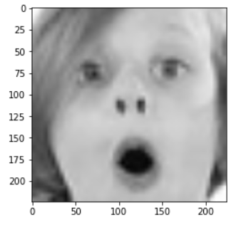
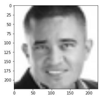
For the purpose of this post, I chose the fer2013 dataset from the Kaggle competition Facial Expression Recognition Challenge from six years ago. The training data consists of 28.709 grayscale images with 48*48 pixel resolution. The target column is an integer indicating one of the 7 emotions, and the pixels column is a space separated string of 2.304 pixels. A rather unusual format for image data if you ask me. To get an idea though, here is two pictures from the dataset:


With the Dataset API, we can load data from many sources including numpy arrays, tensors, text files, csv’s or even folders. In addition, dataset objects come with a handful of nifty methods for data preparation.
.skip(): Most datasets have a header row to be ignored..map(): Map a parse function reshape the dataset to the correct format..shuffle(): Shuffle the data at each iteration to prevent overfitting..repeat(): Repeat the action each iteration..batch(): How many examples to put in each batch..prefetch(): How many batches to prefetch for preprocessing.
Using the last method, preprocessing and model execution will overlap. While the GPU is performing training step n, the CPU will preparing the data for step n+1. This way the GPU is never idle and is constantly fed with new data.
train_dataset=tf.data.TextLineDataset("path/to/train.csv") \
        .skip(1) \
        .map(util.parse_csv) \
        .shuffle(30000) \
        .repeat() \
        .batch(32) \
        .prefetch(1)
The function parse_csv() defines how get from the aforementioned .csv file to tensors. This can be written using TensorFlow functions too.
CSV_COLUMNS=['emotion', 'pixels']
CSV_COLUMN_DEFAULTS=[[0],['']]

def parse_csv(inputs):
    row_columns=tf.expand_dims(inputs, -1)
    columns=tf.decode_csv(row_columns,
                          record_defaults=CSV_COLUMN_DEFAULTS,
                          field_delim=',')
    features=dict(zip(CSV_COLUMNS, columns))

    y=features['emotion']
    y=tf.one_hot(y, depth = 7)
    y=tf.reshape(y, [7])

    x=features['pixels']
    x=tf.string_split(x)
    x=tf.sparse_tensor_to_dense(x, default_value='0') # tf.string_split() outputs a sparse matrix
    x=tf.string_to_number(x)
    x=tf.reshape(x, [48,48,1]) # add channel dimension
    x=tf.image.grayscale_to_rgb(x) # replicate this dimension to get 3 identical channels
    x=tf.image.resize_images(x, [224,224]) # resize image to 224*224

    return x, y
To access this data, we need to define an Iterator. TensorFlow provides a couple of alternatives: Initializable, Reinitializable, One-shot and Feedable. If you want to use both the training as well as the testing data in the same session, the reinitializable iterator is recommended. It enables switching between datasets during the same session. Lastly, the iterator has a get_next() method that yields, well, the next batch.
iterator=tf.data.Iterator.from_structure(train_dataset.output_types,
                                         train_dataset.output_shapes)
x, y=iterator.get_next()

training_init_op=iterator.make_initializer(train_dataset)
validation_init_op=iterator.make_initializer(valid_dataset)

# And now this works:
# model = nets.DenseNet169(x, is_training=is_train, classes=7)
# loss = tf.losses.softmax_cross_entropy(y, model.logits)
Running sess.run(training_init_op) before training and sess.run(validation_init_op) before testing ensures that we are loading the right dataset. Doing data preparation this way, we get rid of the feed_dict mechanism for data ingestion and can plug the values from iterator.get_next() straight into the graph. Last but not least, we should also checkpoint the model’s progress with tf.train.Saver().
with tf.Session() as sess:
       sess.run(init_op)
       sess.run(local_init_op)
       sess.run(training_init_op)
       sess.run(model.pretrained())
       saver = tf.train.Saver()

       for epoch in range(hparams.num_epochs):
             for _ in range(897): # 28709 / 32
                 sess.run(train, {is_train: True})
             # re-initialize the iterator, but this time with validation data
             sess.run(validation_init_op)
             for _ in range(224): # 7178 / 32
                 sess.run(accuracy_op, {is_train: False})

             print("Accumulated validation accuracy is {:.2f}%".format(sess.run(accuracy)*100))
             saver.save(sess, "gs://path/to/ckpt/file" + "{}.ckpt".format(epoch))
To the cloud and back
I could in theory train this on my Macbook Air - perhaps with a batch size of 1 - but why torment my machine when I can outsource the job to Google. Submitting TensorFlow programs to the Cloud ML Engine is easy (and cheap) enough with the gcloud command-line tool. Your training and validation data needs to be uploaded to Google Cloud Storage first. Then, by parametrising the trainer program, you can supply these as additional arguments when submitting the job.
You also need to select a region, resource type, the package-path of your trainer program and the module’s name, a staging bucket on GCS and the path to the tarballs of packages that you need besides the defaults.
Job status can be monitored in the Cloud Console or streamed directly to our terminal with gcloud ml-engine jobs stream-logs jobname.
gcloud ml-engine jobs submit training 'jobname' --region europe-west1 \
                           --scale-tier 'basic-gpu' \
                           --package-path trainer/ \
                           --staging-bucket 'gs://bucketname' \
                           --runtime-version 1.9 \
                           --module-name trainer.task \
                           --python-version 3.5 \
                           --packages deps/Cython-0.29.2.tar.gz,deps/tensornets-0.3.6.tar.gz \
                           -- \
                           --train-file 'gs://bucket name/train.csv' \
                           --eval-file 'gs://bucket name/valid.csv' \
                           ...
Inference and beyond
Once trained, there is a myriad of options to serve a TensorFlow model. Either way, the checkpoint files we saved will need to be transformed. They are useful for restoring model state, but not suited for inference just yet. Weights of the model need to be frozen, training nodes stripped, constants folded (values like batch norms), and overall, we need optimize the model for inference. For an in-depth discussion of these transformations, check out Lukman Ramsey’s awesome article on Medium; here I will solely focus on implementation.
from tensorflow.python.tools import optimize_for_inference_lib
import tensorflow.tools.graph_transforms as graph_transforms
from tensorflow.python.platform import gfile

with tf.Session() as sess:
        saver=tf.train.Saver()
        saver.restore(sess, "path/to/saved_model/model.ckpt")
        # freeze
        frozen_graph_def = tf.graph_util.convert_variables_to_constants(
            sess,
            tf.get_default_graph().as_graph_def(),
            ["densenet169/probs"])
        # transform
        tr_graph_def=graph_transforms.TransformGraph(frozen_graph_def,
                              inputs=["IteratorGetNext"],
                              outputs=["densenet169/probs"],
                              transforms=["strip_unused_nodes",
                              "fold_constants", "fold_batch_norms",
                              "fold_old_batch_norms", "sort_by_execution_order"])
        # optimize
        opt_graph_def = optimize_for_inference_lib.optimize_for_inference(
            tr_graph_def, ["IteratorGetNext"], ["densenet169/probs"],
        tf.float32.as_datatype_enum)

        with tf.gfile.GFile("frozen_graph.pb", "wb") as f:
            f.write(opt_graph_def.SerializeToString())
The result is a .pb file, a protocol buffer in binary format encapsulating the graph definition and the weights. This file is conveniently compatible with the latest version of OpenCV the popular library for computer vision through the function cv2.dnn.readNetFromTensorflow(). A simple program to test the model with a webcam could be as follows:
import numpy as np
import cv2

cap=cv2.VideoCapture(0) # 0 is the webcam device
face_cascade=cv2.CascadeClassifier("face_default.xml") # cascade file to identify face
net=cv2.dnn.readNetFromTensorflow("/path/to/frozen_graph.pb") # read pb file
emotions={0: "Angry",1: "Disgust",2: "Fear",3: "Happy",4: "Sad",5: "Surprise",6: "Neutral"}

while(True):
    ret, frame=cap.read()
    gray=cv2.cvtColor(frame, cv2.COLOR_BGR2GRAY) # turn to gray
    faces=face_cascade.detectMultiScale(frame, 1.3, 5) # detect face

    for (x,y,w,h) in faces:
        cv2.rectangle(frame,(x,y),(x+w,y+h),(255,0,0),2)
        detected_face=gray[int(y):int(y+h), int(x):int(x+w)]# crop detected face
        detected_face=cv2.resize(detected_face, (48, 48)) # resize to 48*48 first to ruin quality
        detected_face=cv2.resize(detected_face, (224, 224)) # resize to 224*224
        gray3c=cv2.cvtColor(detected_face, cv2.COLOR_GRAY2BGR) # make it 3 channels again
        im=np.expand_dims(gray3c, axis=0)

        net.setInput(im.transpose(0, 3, 1, 2), name="IteratorGetNext")
        dnn_out=net.forward("densenet169/probs")

        max_index=np.argmax(dnn_out[0])
        emotion=emotions[max_index]

        cv2.putText(frame, emotion, (int(x), int(y)), cv2.FONT_HERSHEY_SIMPLEX, 1, (255,255,255), 2)

    cv2.imshow('frame', frame)  # Display the resulting frame
    if cv2.waitKey(1) & 0xFF==ord('q'):
        break

cap.release()
cv2.destroyAllWindows()
Running this, the detected expression is displayed above the bounding box for your face.

That’s all folks
Despite the evolution towards high-level API’s, training a modern neural network remains an involved affair. After all, complex models inevitably need more supervision. On the bright side, bleeding edge technology in computer vision or natural language processing is now at the fingertips of the anyone willing to get their hands dirty, and that’s pretty awesome.
For a fully fledged example of what this post described, see the related repo on my GitHub.
G. Huang, Z. Liu , L.vd. Maaten and K.Q. Weinberger. Densely Connected Convolutional Networks, 2016 https://arxiv.org/pdf/1608.06993.pdf↩


