Data prep

First we have to convert policy texts to numbers. A common approach is constructing a document-term matrix where each row is a document and each word is a column. The cells in the matrix contain a statistic about each word in their respective document, such as tf-idf score. It is a simple and powerful way to identify important words in each document. We simply count the number of words per policy and use the number of times it appears in other policies as a weighing factor.

The dimensions of the resulting document-term matrix depend on how many words we include in our vocabulary. Either way, the number of variables will quickly run up to thousands and because most words only appear in a subset of documents, the result will be a sparse matrix. Before anything, let’s split the dataset for modeling.

set.seed(321)
# sample row indices for split
smp_size <- floor(0.75 * nrow(data))
train_ind <- sample(seq_len(nrow(data)), size = smp_size)
# create train and test sets
train <- data[train_ind,]
test <- data[-train_ind,]

To tokenize our text and apply the tf-idf transformations I’ll use the text2vec package. We calculate the tf-idf scores based on the train set, and only map the same values onto the validation set to prevent leakage.

library(text2vec)
library(magrittr)
# exclude stopwords & anything referring to EU
stopwords_gdpr = c(stopwords::stopwords("en"),
                   "gdpr","eu", "eea", 
                   "european", "europe")

# iterators for word level tokenization
it_train <- itoken(train$policy, preprocessor = tolower,
                   tokenizer = word_tokenizer, progressbar = FALSE)
it_test <- itoken(test$policy, preprocessor = tolower,
                  tokenizer = word_tokenizer, progressbar = FALSE)

# create vectorizer function based on iterator and vocab size
vectorizer <- create_vocabulary(it_train, stopwords = stopwords_gdpr) %>%
        prune_vocabulary(doc_count_min = 10, vocab_term_max = 1000) %>%
        vocab_vectorizer()

train_dtm <- create_dtm(it_train, vectorizer)

# tf-idf transformation
tfidf = TfIdf$new()
dtm_train_tfidf = fit_transform(train_dtm, tfidf) # tfidf modified in place!

test_dtm <- create_dtm(it_test, vectorizer)
dtm_test_tfidf = transform(test_dtm, tfidf)

Modeling

Now I’ll train three different models: Regularized logistic regression (glm), support vector machines (svm) and a gradient boosted machines (gbm). The first two are simple linear models remarkably apt at dealing with wide data - remember we have a 1,000 variables; while gbm is a tree-based method considered to be the top of the hill for classifiers. I won’t discuss the internals of these algorithms, and I will only explicitly tune the L1 regularization parameter for the glm (it performs both variable selection as well as coefficient shrinkage, thereby reducing model variance). Hopefully we get respectable performance at first attempt and can jump straight into some explainable machine learning stuffs.

library(caret)
y_train <- factor(train$is_gdpr, levels = c("yes","no"))
y_test <- factor(test$is_gdpr, levels = c("yes","no"))
x_train <- as.data.frame(as.matrix(dtm_train_tfidf))
x_test <- as.data.frame(as.matrix(dtm_test_tfidf))

# boosted trees, glm, svm
# Using caret to perform CV
set.seed(123)
ctrl <- trainControl(method="cv", number=3,classProbs=TRUE)

glm_fit <- train(x = x_train, y = y_train,
                 method="glmnet", trControl = ctrl,
                 tuneGrid = expand.grid(alpha = 1,lambda = seq(0.001,0.1,by = 0.001)))
svm_fit <- train(x = x_train, y = y_train, 
                 method="svmLinear", trControl = ctrl)
gbm_fit <- train(x = x_train, y = y_train, 
                 method="gbm", trControl = ctrl)

Generating predictions for the validation set, let’s plot the performance for the three models:

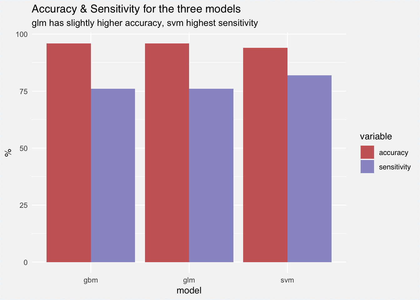
Gbm has the highest accuracy by a inch with around 96%, while svm slightly outperforms the rest with 82% for sensitivity, meaning that 82% of GDPR policies are classified correctly. We are of course most interested what words are differentiating the two classes of policies. We can retrieve measures for variable importance for both the glm as well the gbm models out of the box. For glm we can use varImp(glm_fit) that returns an importance percentage for each variable that’s based on the size of the models coefficients. For gbm we can access the relative influence of each variable using summary(gbm_fit). Relative influence depicts the average empirical improvement of splitting by a variable across all trees generated.

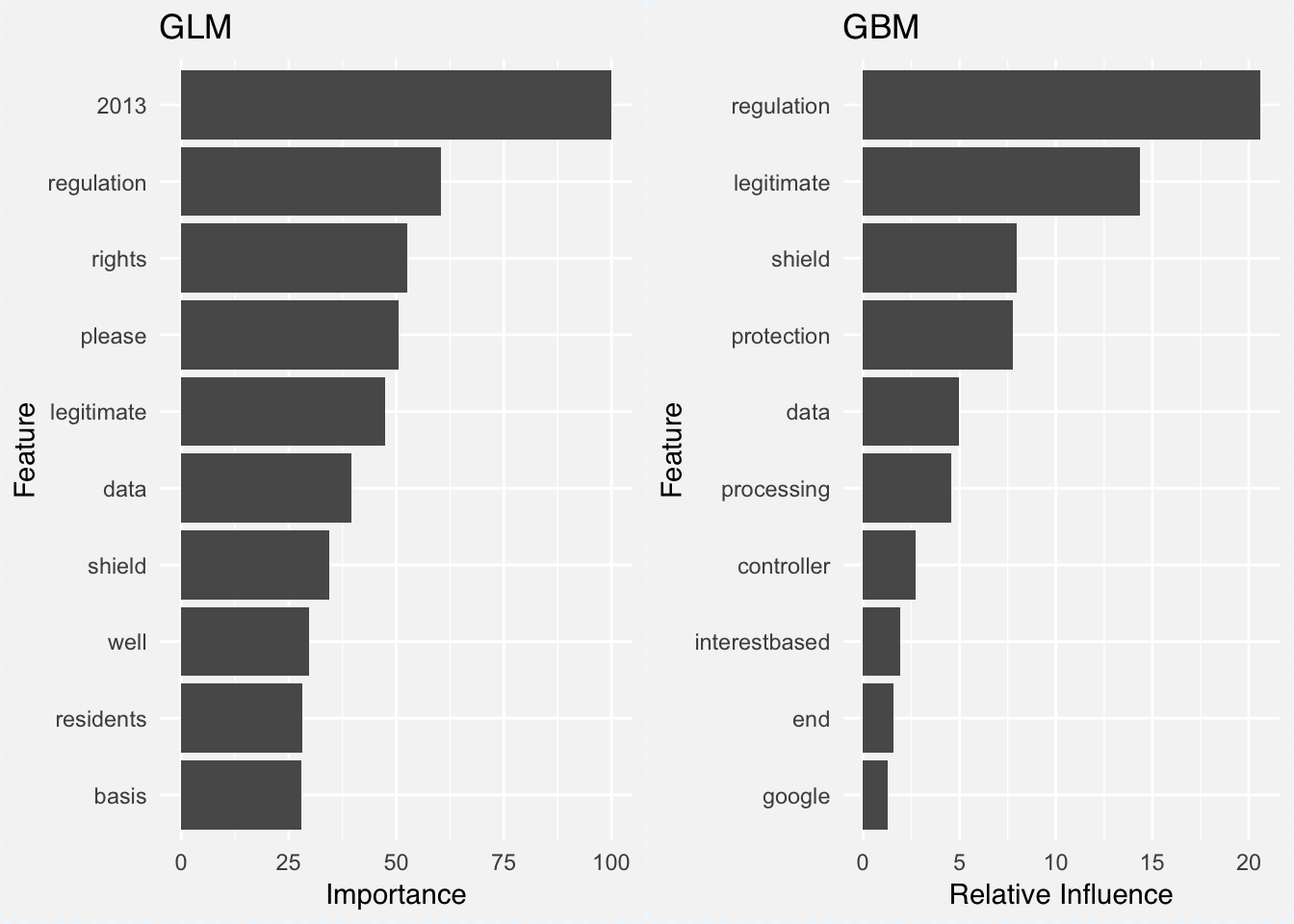
In both cases the word regulation comes out as most important word (I wonder if it has anything to do with GDPRegulation). Other than that, the words data, shield and legitimate appear in both plots for the two models. The problem is of course that we are looking at two different measures for two different models. It would be better to compare the models using the same tools on the same scale using the same metrics.

Descriptive mAchine Learning EXplanations

Article 22 of GDPR states user’s rights to receive information why automated decisions were made and the underlying data processing. Thanks to GDPR, there is a growing interest in developing methods and tools to investigate how predictions are generated by black box models. Enter the world of explainable machine learning frameworks.

One of the newer packages in the field is DALEX, which I learned about at eRum 2018. It has a set of model agnostic tools to investigate what our model is doing. For calculating variable importance:

“… we simply subtract the loss function calculated for validation dataset with permuted values for a single variable from the loss function calculated for validation dataset. This concept and some extensions are described in (Fisher, Rudin, and Dominici 2018).”

Basically we look at how our loss function changes with the permutation of the values in each column. For this we define a prediction and loss function, create an explainer object using explain(), plug into variable_importance() and plot the results.

library(DALEX)
# predict classes
p_fun <- function(object, newdata){
        predict(object, newdata=newdata, type="raw")
}
# accuracy loss, aka error-rate
accuracy_loss <- function(observed, predicted) {
        Metrics::ce(observed, predicted)
}
# explainer object 1
explainer_glm <- explain(glm_fit, label = "glm", data = x_test, 
                         y = y_test, predict_function = p_fun)
# explainer object 2
explainer_svm <- explain(svm_fit, label = "svm", data = x_test, 
                         y = y_test, predict_function = p_fun)
# explainer object 3
explainer_gbm <- explain(gbm_fit, label = "gbm", data = x_test, 
                         y = y_test, predict_function = p_fun)
set.seed(321)
vi_glm <- variable_importance(explainer_glm, loss_function = accuracy_loss, n_sample = -1)
vi_gbm <- variable_importance(explainer_gbm, loss_function = accuracy_loss, n_sample = -1)
vi_svm <- variable_importance(explainer_svm, loss_function = accuracy_loss, n_sample = -1)

plot(vi_glm, vi_svm, vi_gbm)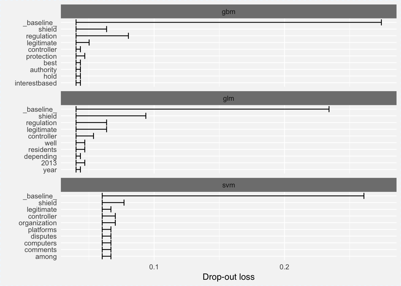

I used error rate (1-accuracy) as the loss function, hence the interpretation of the model is as follows:

• The left edges on the plot represent the error rate of the full model.
• Length of the interval means larger loss -> more important variable.

Looking at the above plot, it confirms that gbm has the lowest overall error rate and there are words shared among the three plots such as shield, controller or regulation that appear in all three plots.

Knowing which variables are important is only the half the story; we would also like to investigate the nature of relationship between the predictor and the prediction. DALEX implements Partial Dependence Plots ² that show how different values of a numeric variable affect the prediction in isolation. We only need to change our prediction function to return probabilities,

p_fun <- function(object, newdata){
        predict(object, newdata=newdata, type="prob")[,1]
}

then rerun our explain() function calls from above, and plug the result into variable_response():

pdp_glm  <- variable_response(explainer_glm, variable = "shield", type = "pdp")
pdp_svm  <- variable_response(explainer_svm, variable = "shield", type = "pdp")
pdp_gbm  <- variable_response(explainer_gbm, variable = "shield", type = "pdp")

plot(pdp_glm, pdp_svm, pdp_gbm)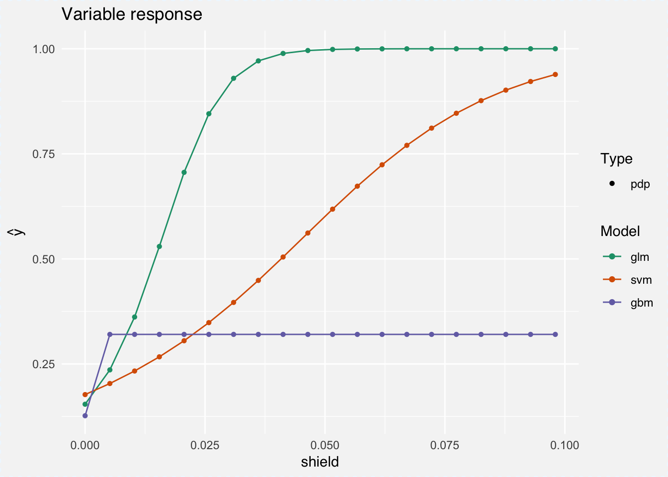

For example, at around a tf-idf score of 0.04 for the word shield, the glm will always predict a GDPR policy. For SVM the cure is lower and the gbm flatlines at a tf-idf score 0.005. One explanation is that our glm model is a lot smaller (thanks to L1 regularization) and so assigns greater weight to important variables. Looking at a couple more words, a similar pattern emerges:

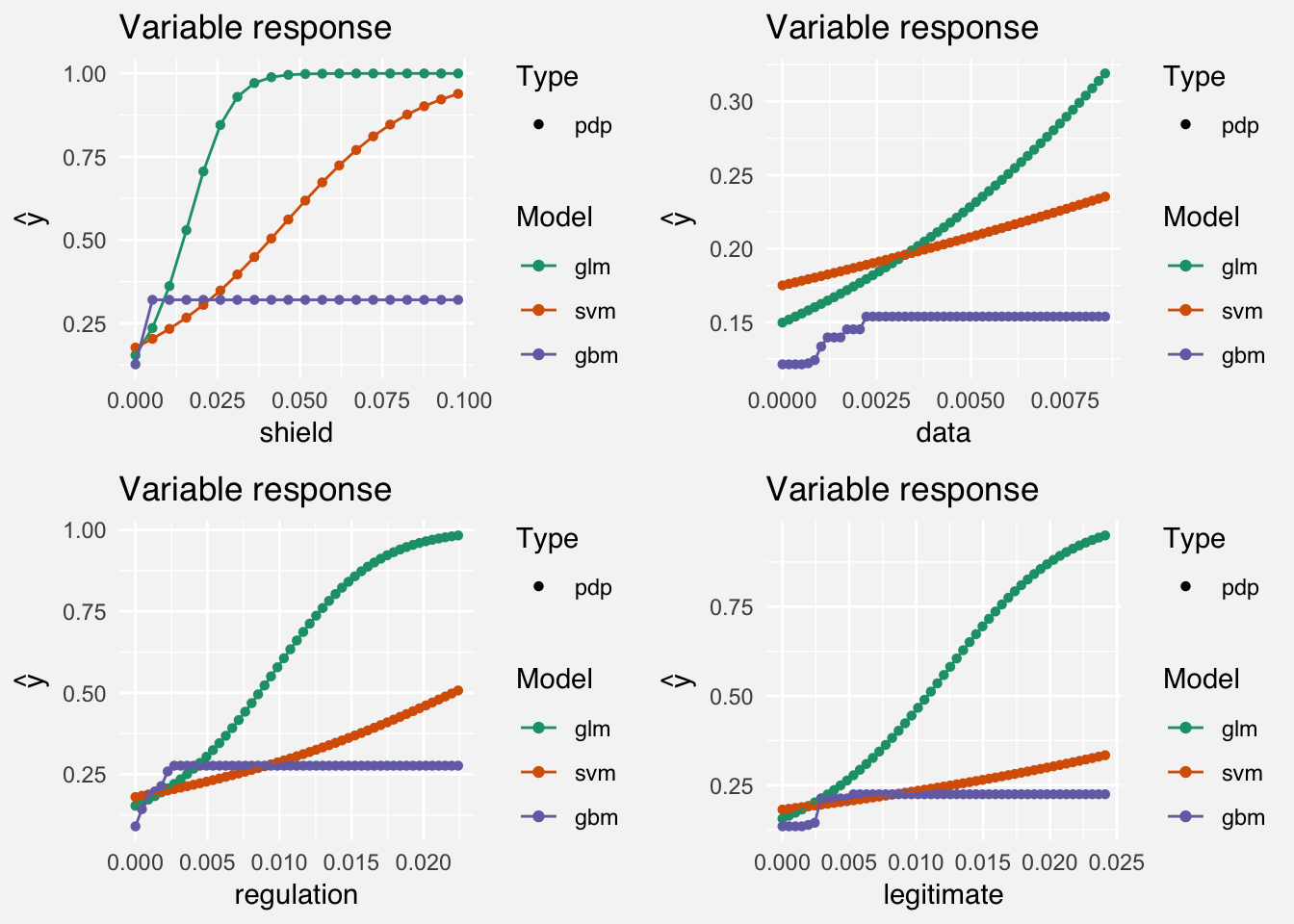
Note that for the words regulation and legitimate, lower tf-idf scores are sufficient for higher probability of being classified as a GDPR policy.