Adventures in the multiverse

For those unfamiliar with the show, Rick and Morty is an animated series about the interuniversal exploits of a half-drunk mad scientist Rick, and his daft grandson Morty. Living under one roof with his daughter, Rick constantly drags his grandson Morty along for adventures into unusual worlds inhabited by surreal creatures. At first hesitant to accompany his eccentric granddad, Morty slowly grows into an indispensable sidekick. Using Rick’s portal gun, they leave the rest of their dysfunctional family at home, and travel through space and time.

Most episodes draw inspiration from or make fun of cult movies such as Back to the Future, A Nightmare on Elm Street, Inception and many other classics by the likes of John Carpenter or David Cronenberg. Besides the ruthless humor and over-the-top visual scenery, the show brilliantly builds independent sci-fi realms, going about their day-to-day according to their wacky rules.

One man’s weekend project, another man’s treasure

After reading the book Tidy Text Mining online, I have been wanting to try out some of the concepts outlined in the book, and the functions of the accompanying package, on an interesting dataset. So I was pretty stoked to find Francois Keck’s subtools package on GitHub, that allows for reading .srt files (the usual format for subtitles) straight into R. With season 3 of Rick and Morty coming to an end last week, the stars have finally aligned to roll up my sleeves and have some fun with text mining.

It is very easy to find English subtitles for pretty much anything on the Internet. With subtools, an entire series can be read with one command from the containing folder, read.subtitles.serie(). We convert the resulting MultiSubtitles object to a data.frame with a second command subDataFrame().

library(subtools)
a <- read.subtitles.serie(dir = "/series/rick and morty/")
df <- subDataFrame(a)
str(df)

## Read: 3 seasons, 31 episodes

## 'data.frame':    16821 obs. of  8 variables:
##  $ ID          : chr  "1" "2" "3" "4" ...
##  $ Timecode.in : chr  "00:00:02.445" "00:00:03.950" "00:00:05.890" "00:00:07.420" ...
##  $ Timecode.out: chr  "00:00:03.850" "00:00:05.765" "00:00:07.295" "00:00:08.925" ...
##  $ Text        : chr  "Morty, you got to... come on." "- You got to come with me. - Rick, what's going on?" "I got a surprise for you, Morty." "It's the middle of the night. What are you talking about?" ...
##  $ season      : chr  "Season_1" "Season_1" "Season_1" "Season_1" ...
##  $ season_num  : num  1 1 1 1 1 1 1 1 1 1 ...
##  $ episode_num : num  1 1 1 1 1 1 1 1 1 1 ...
##  $ serie       : chr  "rick and morty" "rick and morty" "rick and morty" "rick and morty" ...

The $Text column contains the subtitle text, surrounded by additional variables for line id, timestamp, season and episode number. This is the structure preferred by the tidytext package, as it is by the rest of tidyverse.

“Morty, you got to…come on.”

Let’s start with the bread and butter of text mining, term frequencies. We split the text by word, exclude stop words,

data(stop_words)
tidy_df <- df %>%
  unnest_tokens(word, Text) %>%
  anti_join(stop_words)

and aggregate and plot the top 10 words per season.

library(dplyr)
library(ggplot2)

tidy_df %>% group_by(season) %>%
        count(word, sort = TRUE) %>%
        top_n(10) %>%
        ggplot(aes(reorder(word,n), n, fill = season)) +
        geom_col() +
        coord_flip() +
        facet_wrap(~season, scales = "free_y") +
        labs(x = NULL) +
        guides(fill = FALSE) +
        scale_fill_brewer(palette = "Set1")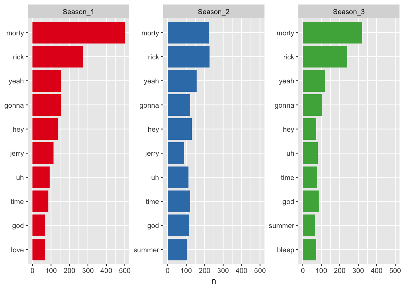

Both seasons are dominated by, well, Rick and Morty. The main characters are tirelessly addressing each other, talking one another either into or out of the mess they find themselves in. What stands out most is the absence of Rick’s daughter, Beth from the top 10 in all seasons. She’s perhaps the only sane person of the family, but then again, sanity doesn’t get too much airtime on this show.

Network analysis on bi-grams

We can similarly get the number of times each two words appear, called bi-grams. Besides calculating summary statistics on bi-grams, we can now construct a network of words according to co-occurrence using igraph, the go-to package for network analysis in R.

library(tidyr)
library(igraph)

bigram_graph <- df %>%
  unnest_tokens(bigram, Text, token = "ngrams", n = 2) %>%
  separate(bigram, c("word1", "word2"), sep = " ") %>%
  filter(!word1 %in% stop_words$word) %>%
  filter(!word2 %in% stop_words$word) %>% 
  group_by(season) %>%
  count(word1, word2, sort = TRUE) %>%
  select(word1, word2, season, n) %>%
  filter(n > 2) %>%
  graph_from_data_frame()

print(bigram_graph)

## IGRAPH 8a11939 DN-- 311 283 -- 
## + attr: name (v/c), season (e/c), n (e/n)
## + edges from 8a11939 (vertex names):
## [1] NA      ->NA      NA      ->NA      NA      ->NA      tiny    ->rick   
## [5] yeah    ->yeah   
##  [ reached getOption("max.print") -- omitted 21 entries ]
## + ... omitted several edges

This igraph object contains a directed network, where the vertices are the words and an edge exists between each that appear after one another more than twice. Representing the text as a graph, we can calculate things such as degree centrality, and plot the results.

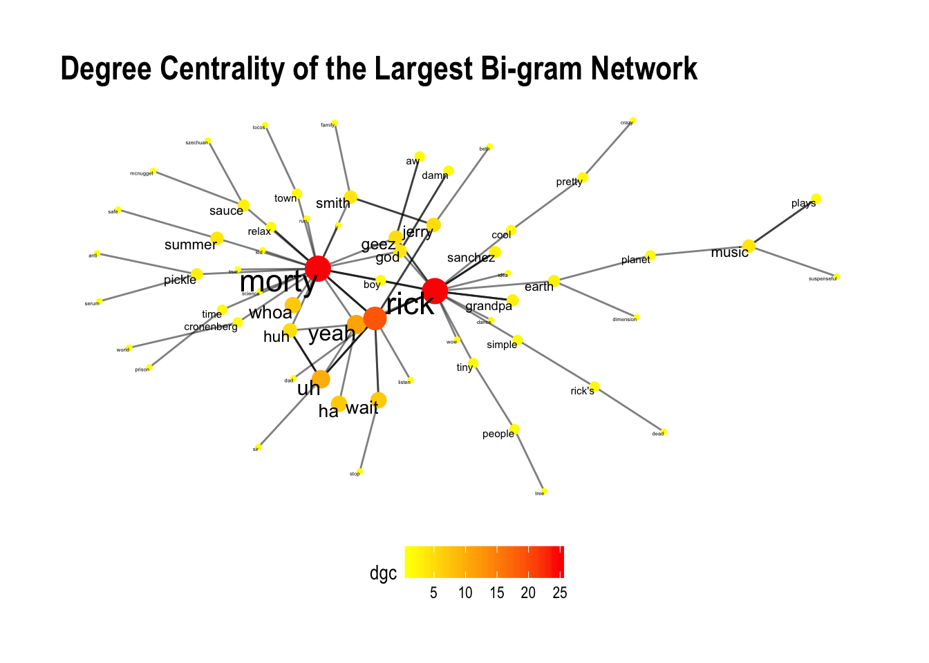
Looking at the largest connected network, we arrive at the same conclusion as with term frequencies. Rick and Morty are the most important words. They are at the center of the network and so have the highest degree centrality scores.

Besides visualising the importance of words in our network, we can similarly differentiate between words that precede either Rick or Morty. These are all the 1st degree connections (words) that have an edge pointing towards the main characters, but aren’t shared among the them.

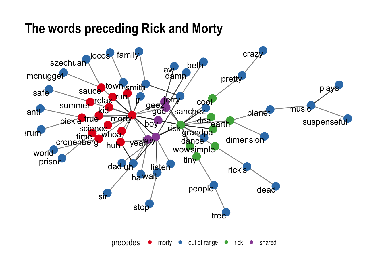
Looking at the red nodes, we recognize many of the things Rick throws at Morty: “Relax Morty!…It’s science Morty!…Run Morty!”. There is also a handful of words that precede both characters like “Geez”, “Boy” or “God”. All other words that are more than one degree away, are colored blue as out of range.

tf-idf

Thus far we have looked at all words across seasons. But where do the seasons differ from each other? And can we summarise each season using a handful of topics? To answer the first question, text mining’s most notorious statistic tf-idf comes to the rescue. It stands for term frequency - inverse document frequency. We take the word counts per season and multiply it by the scaled inverse fraction of seasons that contain the word. Simply put, we penalize words that are common across all seasons, and reward ones that are not. This way, we bring forth the words most typical of each season. Again the tidytext implementation is super easy.

tf_idf_df <- tidy_df %>% 
        count(season, word, sort = TRUE) %>%
        bind_tf_idf(word, season, n)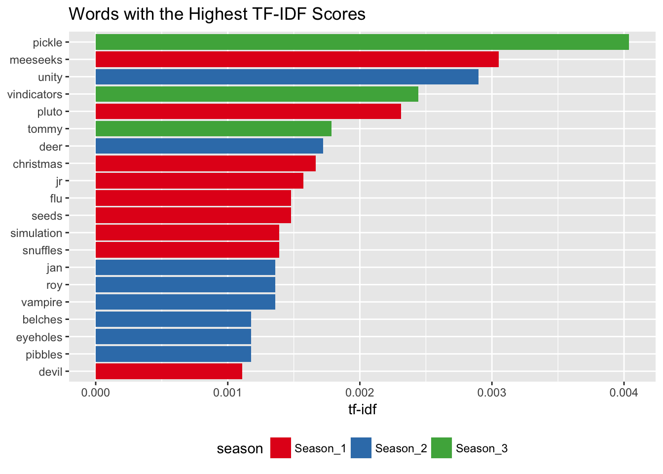

What we get back are the most important elements, characters, motives or places across episodes. I’m somewhat surprised that Mr. Meeseeks didn’t come in first though. I was sure as hell annoyed out of my mind after hearing it uttered for the 100th time during the episode Meeseeks and Destroy. But then again, Mr Meeseeks does make a cameo in two other seasons, so that kind of torpedoes his chances for the first spot.

Topic models

Having seen the most unique words of the script by seasons, we will take our analysis one last step further and try to capture the gist of a the show using topic modeling. Broadly speaking, it’s an unsupervised classification method that tries to represent a document as a collection of topics. Here, I will take the classic Latent Dirichlet Allocation or shortly LDA algorithm for a spin. The basic idea is that

“…a topic is defined as a mixture over words where each word has a probability of belonging to a topic. And a document is a mixture over topics, meaning that a single document can be composed of multiple topics.”"

We could for example take season two, and tell LDA() that we want to compress 10 episodes into just 6 topics. To compensate for the omnipresence of the top words across episodes, I will exclude them for the purpose of clearer separation of topics.

library(topicmodels)
popular_words <- c("rick","morty", "yeah","hey",
                   "summer", "jerry", "uh", "gonna")

episodes_dtm <- tidy_df %>% filter(season_num == 2 & !word %in% popular_words) %>%
        group_by(episode_num) %>%
        count(word, sort = TRUE) %>%
        cast_dtm(episode_num, word, n) 

episodes_lda <- LDA(episodes_dtm, k = 6, control = list(seed = 1234))

After tidy()ing the results, we can plot the top 10 words that contribute (beta) to most to each topic.

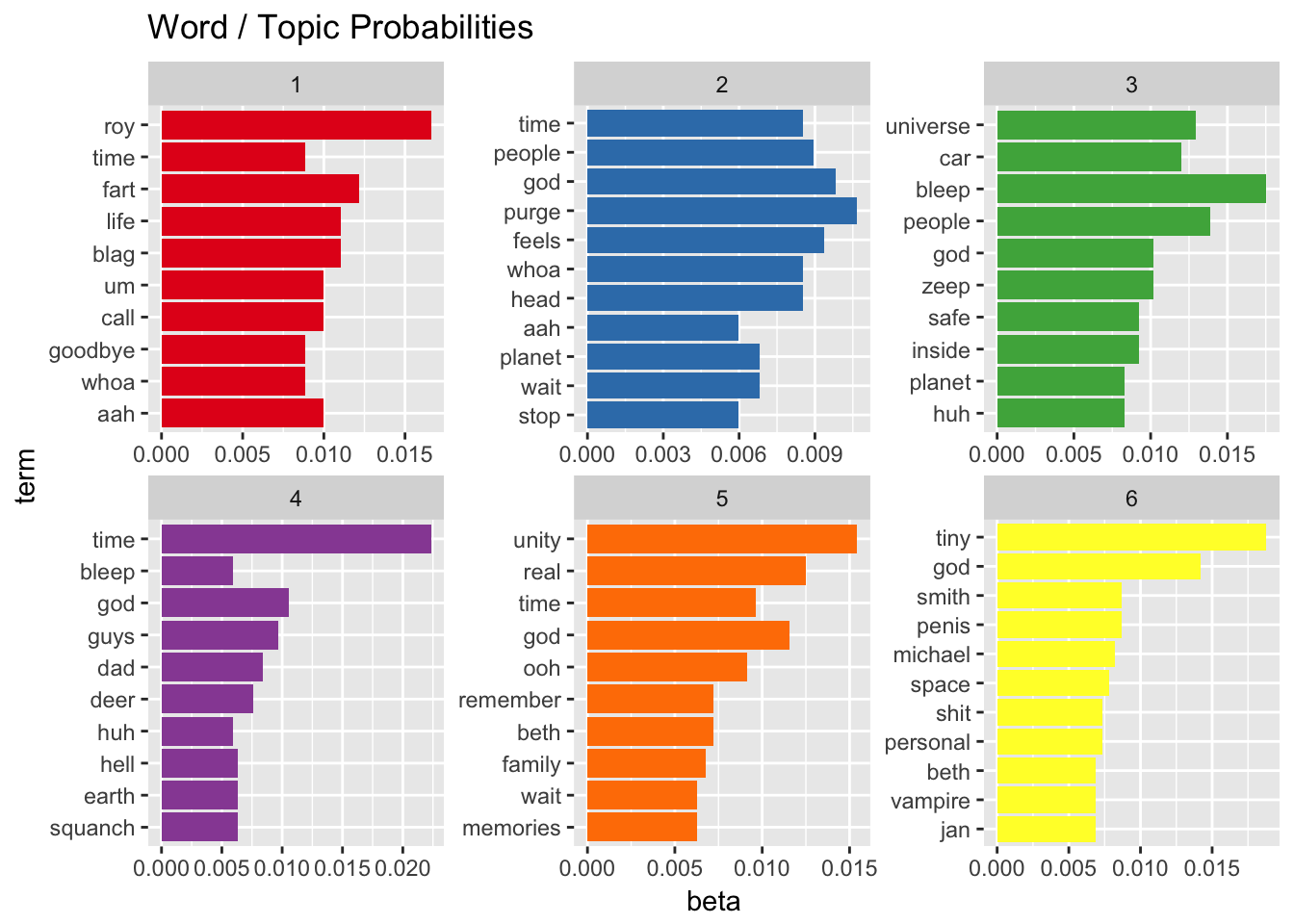
There’s definitely a few topics that contain multiple elements of a particular episode. Take for example topic 1. It includes “Roy”, the name of the videogame Morty plays in the same episode “Fart” appears, a gaseous creature kept under locks by aliens. Or topic 5, which probably relates to the episode where Rick visits his old lover “Unity”. It further contains words as “remember” and “memories”. The episode ends with Unity repeating “I want it real”.

Not only can we examine the word per topic probabilities, we can also plot the topic per document probabilities, or gamma values. This lets us see what topic belongs to what episode.

tidy(episodes_lda, matrix = "gamma") %>%
        inner_join(titles) %>%
        ggplot(aes(factor(topic), gamma)) +
        geom_boxplot() +
        facet_wrap(~ title) +
        ggtitle("Dominant Topics per Episode")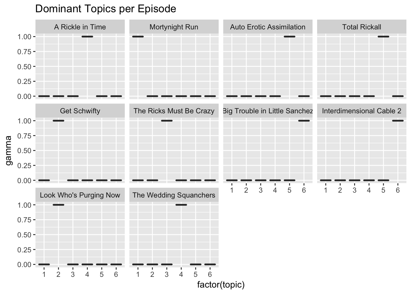

Our previous assumptions are confirmed, the first topic does belong to the episode Mortynight Run as does the fifth topic to Auto-Erotic Assimilation. It is important to note that the results strongly depend on the number of topics supplied to LDA(), so inevitably, some experimentation is required to arrive at meaningful results.

Final thoughts

I ran through some very interesting concepts fairly quickly in this post. I owe much of it to the tidytext package. With very little coding, we can mine a tremendous amount of insights from textual data. And I have just scrachted the surface of what’s possible. The seamless integration with the tidyverse, as with igraph and topicmodels does make a huge difference.

Nonetheless, text mining is a complex topic and when arriving at more advanced material, further reading on the inner workings of these algorithms might come in handy for effective use. The full data and code for this post is available as usual on my Github.